Serialization 101
Welcome to Serialization 101. This course is a starting point for anyone who wants to understand data serialization. You do not need prior experience with distributed systems, data lakes, or binary formats. First-year students, data scientists, and working engineers can all begin here.
| Jump | |
|---|---|
| This track | Three lenses below · then 201 mechanisms |
| See numbers | Dashboard · language Overview for roster |
| How we measure | Benchmarks |
By the end of this theory track you should be able to:
- Explain what serialization is and why computer programs need it.
- Read the history of data formats as answers to real problems, not as a list of product names.
- Choose a format for a specific kind of work by using the right lens. One lens is data work. Another lens is services and systems.
- Connect the ideas in these pages to measured libraries in this multi-language benchmark suite.
- Name the standard a library implements, and tell that name apart from the family it belongs to.
Theory alone does not tell you what to ship in production. Use this course to build vocabulary and judgment. Then check real numbers on the Dashboard. Language Overview pages list the roster and caveats. For how those numbers are produced, see Benchmarks.
What is serialization?
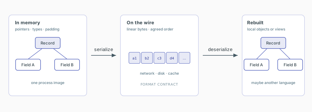
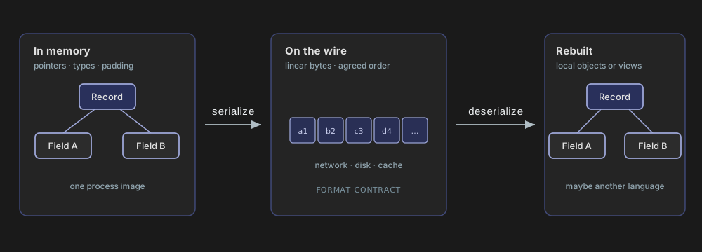
Serialization is the process of turning an in-memory data structure into a linear sequence of bytes. Those bytes can be stored on disk, held in a cache, or sent across a network. Deserialization is the reverse process. It rebuilds a usable structure from those bytes. The rebuilt structure may live in another process, on another machine, or in another programming language.
Why is this necessary? Inside a running program, data is often a web of pointers and types. A record may point to an array. That array may point to strings. Those strings may point to characters. Networks and disks do not understand that web. They only store and transmit bytes in order. Every serialization format is therefore a contract between a writer and a reader. The contract says how the web of meaning is flattened into bytes. It also says how those bytes are rebuilt later.
Three lenses
The same formats appear under three perspectives on purpose. Each document answers a different question:
| Lens | Primary question | Best if you care about… |
|---|---|---|
| Historical | Why do these formats exist? | Eras, people, constraints, and major shifts in thinking |
| Data science | What should I use for data and machine-learning work? | Lakes, pipelines, notebooks, models, and columnar input/output |
| Engineering | What should I ship in services and systems? | APIs, remote procedure calls (RPC), performance, security, and long-term change |
Suggested order for a first pass
- Skim the shared trade-offs below. This takes about ten minutes.
- Read the historical perspective once for the big picture.
- Deep-dive the lens that matches your work. Choose either data science or engineering.
- Open Serialization categories. Also open a language Overview (roster) and the Dashboard (numbers) for libraries you might actually use. On the Dashboard, set Language, Standard, Data set, and Data type before you read a ranking. That combination is the comparison cell.
- When you need mechanisms (how formats work under the hood), work through the Serialization 201 track:
- Memory layout. If a value is narrower than a byte, or someone argues that a wide bus should change the format, continue with the optional page Bit width is not bus width.
- Encode/decode cost
- Self-describing vs schema
- Schema evolution
- Dynamic vs IDL binary
- Zero-copy
- Compression vs format
You can reverse steps 2 and 3 if you already have a concrete problem. For example, you might need Parquet for analytics, or an internal service format. Jump to a single 201 article when you already know the question you want answered.
When the mechanisms feel solid and you need production judgment under several constraints at once, continue to Serialization 301.
Core trade-offs
These axes appear in every lens. Learn the names here. The perspective documents fill in the details.
Text versus binary
| Text (JSON, XML, YAML, and similar) | Binary (MessagePack, Protocol Buffers, Parquet, and similar) | |
|---|---|---|
| Strength | Humans can read it. It is easier to debug and log. | Compact. Often much faster to encode and decode. |
| Cost | Larger payloads. Parsing character by character is slower. | Opaque without tools. Harder to inspect by hand. |
In other words, text formats trade size and speed for readability. Binary formats trade readability for density and often for speed.
Schema versus schemaless
A schema is a written description of the shape of the data. It says which fields exist, what types they have, and how they may change over time.
| Schemaless (JSON, MessagePack, and similar) | Schema-driven (Protocol Buffers, Avro, FlatBuffers, and similar) | |
|---|---|---|
| Strength | Flexible. You can ship data without an interface-description step. | Compact on the wire. Supports code generation. Clearer evolution rules when you invest in process. |
| Cost | Validation and compatibility are your job. | Up-front schema design and tooling. |
Row-oriented versus columnar
| Row (JSON objects, Protocol Buffers messages, Avro records) | Columnar (Parquet, ORC, Arrow tables) | |
|---|---|---|
| Strength | Natural for whole records. Fits APIs, RPC, and online transaction-style access. | Scan a few columns over huge tables with far less input/output. |
| Cost | Poor for wide analytical queries. | Wrong default when you mostly fetch one document by id. |
Think of a spreadsheet. A row-oriented format stores one complete row after another. A columnar format stores all values of column A together, then all values of column B, and so on. Analytics queries that touch only a few columns benefit from the columnar layout.
Self-describing versus schema-dependent
- Self-describing (to varying degrees): Field names or type tags travel with the data. JSON, MessagePack, and CBOR are examples. These formats are easier to inspect. They also carry more metadata on the wire.
- Schema-dependent: The wire data is nearly meaningless without a shared schema. Classic Protocol Buffers and raw Avro work this way. These formats are smaller and faster when both ends already agree on the contract.
Portable versus language-native
- Portable: Designed for multi-language interchange. JSON, Protocol Buffers, MessagePack, and similar formats fit here.
- Language-native: Tied to one runtime. Examples include
pickleand Java serialization. These are convenient inside a tight trust boundary. They are dangerous or unusable across languages. They are also unsafe on untrusted inputs.
A trust boundary is any place where data leaves a fully controlled environment and may be influenced by someone else. A public network request is one example.
Family, standard, and library
The five axes above describe the job. The Dashboard filters by the standard’s name.
A family is a teaching cut. It groups formats by the job: text, schemaless binary, schema-driven, language-native, or columnar. Serialization categories is that map. A family is not a Dashboard filter.
A standard is a named contract, such as JSON, Avro, or Arrow IPC. Several libraries can implement one standard. The Dashboard Standard control is that name. The compliance catalog is where each name is defined.
A library is one implementation of a standard in one language. orjson and Python’s json module are both the JSON standard. The speed gap between them is the library.
The comparison cell is language, standard, data set, and data type. Data set is Suite, Columnar, or Graph. The Suite types are message, document, telemetry, strings, and event. Published averages such as all@all use only those five types. The Columnar types are table, table_project, nested_table, and signal. On table_project, serialize writes the full row and deserialize reads only the column f_float_0. The Graph type is graph (shared nodes and one reference cycle). It is not part of all@.
| Pair | Family | Standards |
|---|---|---|
| JSON and YAML | Text | JSON and YAML |
| Protocol Buffers and Avro | Schema-driven | Protocol Buffers and Avro |
| Arrow IPC, Parquet, and ORC | Columnar | Arrow IPC, Parquet, and ORC |
SBE (Simple Binary Encoding) keeps the three labels separate. It sits in the schema-driven family. Its data set is Columnar. Its standard is SBE. Each record is one stride: the bytes from the start of that record to the start of the next. Variable-length fields change that distance. SBE is not a columnar file format like Parquet.
Libraries with no public spec, such as pickle, bincode, and the in-tree custom binaries, use the Dashboard standard No public spec on Overview, Compare, and Compliance. Compliance does not score them.
Lab notebooks (Python / Colab)
Hands-on companions for two of the lenses:
| Notebook | Article |
|---|---|
| Data science lab | Data science perspective |
| Engineering mini lab | Engineering perspective |
Install and layout notes live in the notebooks README.
Scope and honesty
- This theory track is a map, not an encyclopedia of every library.
- Performance claims in prose are illustrative. Prefer the Dashboard for numbers on this benchmark runner and hardware.
- “Best format” always means best under your constraints. Those constraints include team skills, trust boundaries, retention needs, latency budgets, and multi-language requirements.